The Application of Quantitative Energy Dispersive Spectroscopy to Amphibole (Mineral) Identification in the Regulatory Field
Frank M Craig

The complete characterization (identification) of a mineral typically requires more than a day of work using more than one analytical technique. Most analysts in the regulatory field are not afforded such a luxury. More often than not, identification is required within hours of receiving a sample (including preparation time). The most common technique currently in use to provide this identification is Analytical Transmission Electron Microscopy (ATEM) – a TEM with an Energy Dispersive Spectrometer attached.

Energy Dispersive Spectroscopy (EDS) is the quickest and easiest way to identify the primary constituents (ions) of a mineral irradiated by an electron beam. However, there are many limitations to its use. First, the electron microprobe (both EDS and wavelength dispersive spectroscopy (WDS)) is designed for the analysis of materials with a smooth, polished surface; particles rarely have flat, smooth surfaces. The edge effects resulting from a rough surface will influence the signal and consequently the (semi) quantitative data. The second is the way EDS handles data.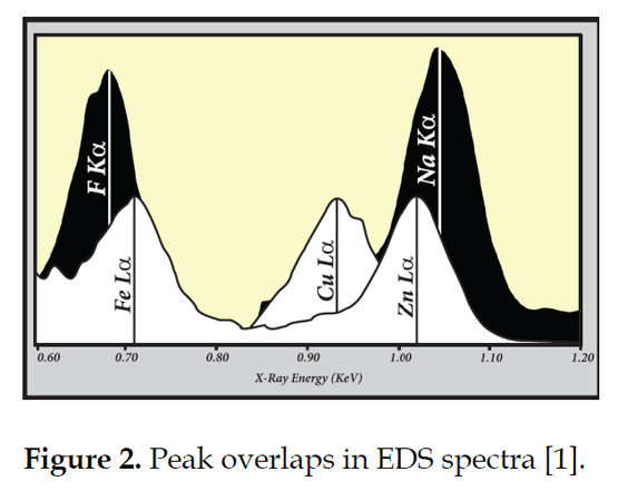 Semi-quantitative data are typically ‘forced’ to total 100%. Among other factors, this is a problem when it comes to the amphiboles as these minerals are hydrated and can include lithium. Both are not accounted for by the scan and so the analysis will not truly total 100%. A third limitation is peak overlaps, multiple elements with the same or similar energies, within the spectra (Fig. 2). These overlaps affect both the qualitative and quantitative interpretation of the spectra. There can be enough of a non-essential element that its peak completely obscures and/or alters the weight of an essential element.

The chemistry of the mineral will also factor into the interpretation. Part of the definition of a mineral is that it have a specific chemical composition. Realistically, this translates to a narrow range of compositions. Amphiboles are among the most difficult to distinguish in this respect as complex ion exchange vectors lead to a continuum of compositions between two ideal end-members known as a solid solution. This exchange of elements is not random, but controlled by a few basic rules of coupled substitutions and/or element-by-element substitutions [2]. The International Mineralogical association (IMA) nomenclature [3, 4] deals with this complexity by utilizing the ‘50%’ rule, with approved prefixes. Take, as an example, the amphibole tremolite – end member formula of Ca₂Mg₅Si₈O₂₂(OH)₂. A common exchange vector in this series (and all amphiboles) is Mg⁺² <-> Fe⁺² which can be complete leading to the opposite end member: ferro-actinolite – Ca₂Fe₅Si₈O₂₂(OH)₂. Since every combination in between is possible, the formula is often written as Ca₂(Mg,Fe)₅Si₈O₂₂(OH)₂. Tremolite is defined as the composition with less than 50% iron (actinolite is no longer a valid name under the current nomenclature [4], but is ‘grandfathered’ and retained with the definition of iron between 0.5 and 2.5 apfu in the C-site). Let’s make things a little more interesting by considering an (OH)^-1 <-> F^-1 substitution. Again, more than 50% fluorine and the name becomes fluor-tremolite (etc.): i.e. Ca2(Mg,Fe)5Si8O22(OH,F)2. These sometimes subtle differences are important because, at this time, only tremolite-asbestos and actinolite-asbestos are regulated.

Compositional zoning and/or exsolution (Fig. 3) within a crystal can further complicate the issue. The simple definition of zoning is a chemical variation from the core of a crystal to its rim: a crystal that has a core with one composition grading to a rim with another composition. Exsolution is a process where a single solid-solution phase separates or un-mixes into two or more phases in the solid state. Both zoning and exsolution only occur in minerals whose composition varies between two (or more) pure endmembers (a solid solution).

The IMA currently recognizes over 100 amphibole species which are classified based on their chemical make-up; not only what ions are present but also what atomic sites within the lattice these ions occupy (Fig. 4). The current nomenclature [4] changed the classification dramatically. Amphibole was elevated to super group status with two groups of minerals defined based on the dominant W site anion: the (OH, F, Cl) dominant and the (O) dominant groups. The (OH, F, Cl) group is further divided into eight subgroups based on the dominant B cation. The regulatory field is only concerned with four: calcic, calcic-sodic, sodic, and magnesium-iron-manganese groups. However, the quantification of Fe+3 plays a key role in this new classification. This is a problem because Fe+3 cannot be quantified with the electron microprobe (EDS or WDS). A value for Fe+3 can be estimated with a number of assumptions and associated errors (an error of up to 30% has been documented) [5]. The 1997 IMA classification [3] is probably the more appropriate scheme for the regulatory field. The difference between the two schemes can be significant (Fig. 5). Currently, the nomenclature used is at the discretion of the analyst.




















Site assignments are relatively straightforward once a composition has been obtained (Fig. 6). Generally, it’s easiest to work right to left and assign the T site first (the W site is assumed to be occupied by (OH) only). Silica is ordered preferentially followed by Al then Ti. Here Si plus Al fills the T site. The remaining Al is placed in the C site. Magnesium is then ordered preferentially, here all of the Mg is placed into C with Fe⁺² completing the site. The remaining Fe⁺² will go into the B site with calcium completing the site.

A normalized composition will have a total of 15 to 16 cations [3, 4]. There are only a few possibilities, analytical (instrument) error aside, that a composition will not normalize (an error of +/- 0.1 apfu is generally considered as acceptable). First, the mineral analyzed is not an amphibole. There are a number of minerals that have spectra which look similar to a regulated amphibole, most notably talc and the pyroxenes [1]. Second, there are ions (valences) present that were not included in the analysis. EDS cannot detect lithium (which can be present in amphiboles) or the valence state of an ion. Consider iron, a common constituent of amphiboles, as an example. There are three valance states of iron: Fe⁺², Fe⁺³, and Fe⁺⁴. EDS will only tell you that iron is present, traditionally reported as FeO. Such absences will not only impact the site assignment where the error originated, but also the other site assignments. The sodic amphiboles, as an example, are notorious for having both ferro (+2) and ferri (+3) iron in the same mineral. Since only one can be quantified, the absence of the other (plus the possible presence of lithium) will throw off the final normalization. This error usually manifests as one site being ‘light’ which is compensated for by another site being ‘heavy’ (Fig. 7). A third possibility is the normalization technique. The IMA nomenclature uses the anion normalization of either 23 or 24 oxygens. This is somewhat of a problem as the true number of oxygen ions cannot be determined from an EDS scan. The (OH) anion group may be partially or completely replaced by fluorine, chlorine, or oxygen. Since cations are measured directly, many mineralogists and petrologists prefer a cation-based scheme with the anion scheme employed as a last resort. Both techniques have positives and negatives, the one used is at the discretion of the analyst.

Considered by some to be a substandard analytical technique, (semi) quantitative EDS does show merit for the identification of the amphibole minerals commonly encountered by regulatory scientists, i.e minerals like the tremolite-ferro-actinolite series or the grunerite-cummingtonite and anthophyllite-gedrite series. Quantitative EDS can even be used for some members of the hornblende and sodic-calcic groups. EDS can also be used to identify other minerals that may be encountered during a routine analysis such as the pyroxene group or other inosilicates (Fig. 8).


There are a few advantages to using EDS as a tool for mineral identification - ease of use and speed are the two biggest. Only a few of the limitations have been discussed here. The user does need to be aware of all possible sources of error when interpreting an EDS scan. Even in the event the data do normalize to an ideal formula (Fig. 9), EDS and WDS data should never be used alone to positively identify a mineral. Modern electron microscopes are capable of diffraction (Fig. 10) and when combined with the microprobe data will confirm the identification. Any positive identification in the absence of diffraction is the judgement of the analyst.


References
[1] Craig. F. M., 2017, Asbestos Characterization: TEM Atlas of Regulated and Select Interference Minerals, 2nd Edition:

[2] Revheim, O., 2017, The Amphiboles, an Introduction: Unpublished Manuscript: 12 p.

[3] Leake, B. E., A. R. Woolley, C.E.S. Arps, W. D. Birch, M. C. Gilbert, J. D. Grice, F. R. Hawthorne, A. Kato, H. J. Kisch, V. G. Krivoviche, K. Linthout, J. Laird, J. A. Mandarino, W. V. Maresch, E. H. Nickel, N. M. S. Rock, J. C. Schumacher, D. C. Smith, N. C .N. Stephenson, L. Ungaretti, E. J. W. Whittaker and G. Youzhi, 1997, Nomenclature of the Amphiboles: Report of the Subcommittee on Amphiboles of the International Mineralogical Association, Commission on New Minerals and Mineral Names: The Canadian Mineralogist, v. 35, p. 219 – 246.

[4] Hawthorne F. R., Oberti, G. E Harlow, W. V. Maresch, R. F. Martin, J.C. Schumacher and M. D. Welch, 2012, Nomenclature of the Amphibole Supergroup: American Mineralogist, v. 97, p. 2031–2048.

[5] Lamb, W. M., R, Guillemette, R. K. Popp, S. J. Fritz and G. J. Chmiel, 2012, Determination of Fe3+/Fe using the electron microprobe: A calibration for amphiboles: American Mineralogist, v. 97, p. 951 - 961.